Compute time delay estimates

This example demonstrates how time delay estimation (TDE) can be computed with PyBispectra.

# Author(s):
#   Thomas S. Binns | github.com/tsbinns

import numpy as np

from pybispectra import compute_fft, get_example_data_paths, TDE

Background

A common feature of interest in signal analyses is determining the flow of information between two signals, in terms of both the direction and the particular time lag between them.

The method available in PyBispectra is based on the bispectrum, \(\textbf{B}\). The bispectrum has the general form

\(\textbf{B}_{kmn}(f_1,f_2)=<\textbf{k}(f_1)\textbf{m}(f_2)\textbf{n}^* (f_2+f_1)>\) ,

where \(kmn\) is a combination of signals with Fourier coefficients \(\textbf{k}\), \(\textbf{m}\), and \(\textbf{n}\), respectively; \(f_1\) and \(f_2\) correspond to a lower and higher frequency, respectively; and \(<>\) represents the average value over epochs. When computing time delays, information from \(\textbf{n}\) is taken not only from the positive frequencies, but also the negative frequencies.

Four methods exist for computing TDE based on the bispectrum [1]. The fundamental equation is as follows

\(\textrm{TDE}_{xy}(\tau)=\int_{-\pi}^{+\pi}\int_{-\pi}^{+\pi}\textbf{I} (\textbf{x}_{f_1},\textbf{y}_{f_2})e^{-if_1\tau}df_1df_2\) ,

where \(\textbf{I}\) varies depending on the method; and \(\tau\) is a given time delay. Phase information of the signals is extracted from the bispectrum in two variants used by the different methods:

\(\boldsymbol{\phi}(\textbf{x}_{f_1},\textbf{y}_{f_2})= \boldsymbol{\varphi}_{\textbf{B}_{xyx}} (f_1,f_2)-\boldsymbol{ \varphi}_{\textbf{B}_{xxx}}(f_1,f_2)\) ;

\(\boldsymbol{\phi}'(\textbf{x}_{f_1},\textbf{y}_{f_2})= \boldsymbol{\varphi}_{\textbf{B}_{xyx}}(f_1,f_2)-\frac{1}{2}( \boldsymbol{\varphi}_{\textbf{B}_{xxx}}(f_1,f_2) + \boldsymbol{ \varphi}_{\textbf{B}_{yyy}}(f_1,f_2))\) .

Method I: \(\textbf{I}(\textbf{x}_{f_1},\textbf{y}_{f_2})=e^{i\boldsymbol{ \phi}(\textbf{x}_{f_1},\textbf{y}_{f_2})}\)

Method II: \(\textbf{I}(\textbf{x}_{f_1},\textbf{y}_{f_2})=e^{i\boldsymbol{ \phi}'(\textbf{x}_{f_1},\textbf{y}_{f_2})}\)

Method III: \(\textbf{I}(\textbf{x}_{f_1},\textbf{y}_{f_2})=\Large \frac{ \textbf{B}_{xyx}(f_1,f_2)}{\textbf{B}_{xxx}(f_1,f_2)}\)

Method IV: \(\textbf{I}(\textbf{x}_{f_1},\textbf{y}_{f_2})=\Large \frac{ |\textbf{B}_{xyx}(f_1,f_2)|e^{i\boldsymbol{\phi}'(\textbf{x}_{f_1}, \textbf{y}_{f_2})}}{\sqrt{|\textbf{B}_{xxx}(f_1,f_2)||\textbf{B}_{yyy} (f_1,f_2)|}}\)

where \(\boldsymbol{\varphi}_{\textbf{B}}\) is the phase of the bispectrum. All four methods aim to capture the phase difference between \(\textbf{x}\) and \(\textbf{y}\). Method I involves the extraction of phase spectrum periodicity and monotony, with method III involving an additional amplitude weighting from the bispectrum of \(\textbf{x}\). Method II instead relies on a combination of phase spectra of the different frequency components, with method IV containing an additional amplitude weighting from the bispectrum of \(\textbf{x}\) and \(\textbf{y}\). No single method is superior to another. If time delay estimates for only certain frequencies are desired, this information can be extracted from the matrix \(\textbf{I}\).

As a result of volume conduction artefacts (i.e. a common underlying signal that propagates instantaneously to \(\textbf{x}\) and \(\textbf{y}\)), time delay estimates can become contaminated, resulting in spurious estimates of \(\tau=0\). Thankfully, antisymmetrisation of the bispectrum can be used to address these mixing artefacts [2], which is implemented here as the replacement of \(\textbf{B}_{xyx}\) with \((\textbf{B}_{xyx} - \textbf{B}_{yxx})\) in the above equations [3].

Loading data and computing Fourier coefficients

We will start by loading some simulated data containing a time delay of 250 ms between two signals, where \(\textbf{y}\) is a delayed version of \(\textbf{x}\). We will then compute the Fourier coefficients of the data, which will be used to compute the time delay.

We specify n_points to be twice the number of time points in the data, plus one. This ensures that the time delay estimate spectrum is returned for the whole epoch length (in both positive and negative delay directions, i.e. where \(\textbf{x}\) drives \(\textbf{y}\), and \(\textbf{y}\) drives \(\textbf{x}\)) with the same temporal resolution as the original data. Using a number of points smaller than this will reduce the window in which time delay estimates can be computed below the epoch length, whereas using a higher number of points will only artificially increase this window length. Accordingly n_points=2 * n_times + 1 is recommended.

In this example, our data consists of 30 epochs of 200 timepoints each, which with a 200 Hz sampling frequency corresponds to 1 second of data per epoch (one timepoint every 5 ms). Note that the temporal resolution of the time delay estimates can be increased by increasing the sampling rate of the data.

# load simulated data
data = np.load(get_example_data_paths("sim_data_tde_independent_noise"))
sampling_freq = 200  # sampling frequency in Hz
n_times = data.shape[2]  # number of timepoints in the data

# compute Fourier coeffs.
fft_coeffs, freqs = compute_fft(
    data=data,
    sampling_freq=sampling_freq,
    n_points=2 * n_times + 1,  # recommended for time delay estimation
    window="hamming",
    verbose=False,
)

print(
    f"FFT coeffs.: [{fft_coeffs.shape[0]} epochs x {fft_coeffs.shape[1]} "
    f"channels x {fft_coeffs.shape[2]} frequencies]\nFreq. range: "
    f"{freqs[0]:.0f} - {freqs[1]:.0f} Hz"
)

FFT coeffs.: [30 epochs x 2 channels x 201 frequencies]
Freq. range: 0 - 0 Hz

Computing time delays

To compute time delays, we start by initialising the TDE class object with the Fourier coefficients and the frequency information and call the compute() method. For simplicity, we will focus on TDE using method I. To demonstrate that TDE can show the directionality of information flow as well as the particular time lag, we will compute TDE from signals 0 -> 1 (the genuine direction of information flow where the time delay should have a positive value) and from signals 1 -> 0 (the reverse direction of information flow where the time delay should have a negative value).

Using the fmin and fmax arguments, time delay information for frequency band(s) of interest can be isolated by specifying the lower and higher frequencies of interest. Here, we will compute time delays for all frequencies. Performing time delay estimation on frequency bands is discussed in the following example: Compute time delay estimates for frequency bands.

tde = TDE(
    data=fft_coeffs, freqs=freqs, sampling_freq=sampling_freq, verbose=False
)  # initialise object
tde.compute(indices=((0, 1), (1, 0)), method=1)  # compute TDE
tde_times = tde.results.times

tde_results = tde.results.get_results()  # return results as array

print(
    f"TDE results: [{tde_results.shape[0]} connections x "
    f"{tde_results.shape[1]} frequency bands x {tde_results.shape[2]} times]"
)

TDE results: [2 connections x 1 frequency bands x 401 times]

We can see that time delays have been computed for two connections (0 -> 1 and 1 -> 0) and one frequency band (0-100 Hz), with 401 timepoints, and averaged across our 30 epochs. The timepoints correspond to time delay estimates for every 5 ms (i.e. the sampling rate of the data), ranging from -1000 ms to +1000 ms.

Plotting time delays

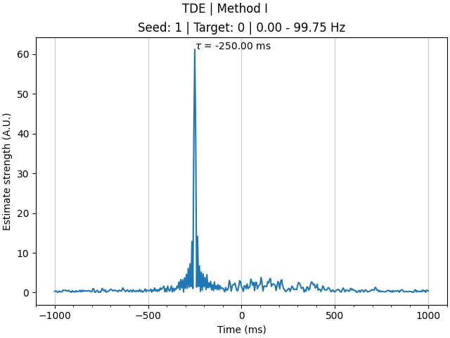
Let us now inspect the results. Note that the Figure and Axes objects can be returned for any desired manual adjustments of the plots. When handling TDE results, we take the time at which the strength of the estimate is maximal as our \(\tau\). Doing so, we indeed see that the time delay is identified as 250 ms. Furthermore, comparing the two connections, we see that the direction of information flow is also correctly identified, with the result for connection 0 -> 1 being positive and the result for connection 1 -> 0 being negative (i.e. information flow from signal 0 to signal 1). Here, we manually find \(\tau\) based on the maximal value of the TDE results, however this information is also precomputed and can be accessed via the tau attribute.

Taking the time at which the estimate is maximal as our \(\tau\) is one approach to use when estimating time delays. For interest, however, we can also plot the full time course of the TDE results. In this low noise example, we see that there is a clear peak in time delay estimates at 250 ms. Depending on the nature and degree of noise in the data, the time delay spectra may be less clear, and you may find advantages using the other TDE method variants.

print(
    "The estimated time delay between signals 0 and 1 is "
    f"{tde_times[tde_results[0].argmax()]:.0f} ms.\n"
    "The estimated time delay between signals 1 and 0 is "
    f"{tde_times[tde_results[1].argmax()]:.0f} ms."
)

for con_i in range(tde_results.shape[0]):
    assert tde_times[tde_results[con_i].argmax()] == tde.results.tau[con_i]

fig, axes = tde.results.plot()

• 
• 

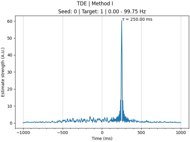
The estimated time delay between signals 0 and 1 is 250 ms.
The estimated time delay between signals 1 and 0 is -250 ms.

Handling artefacts from volume conduction

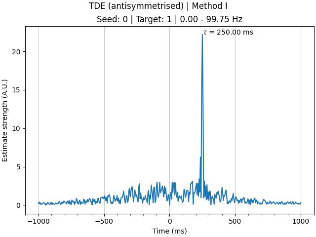
In the example above, we looked at simulated data from two signals with independent noise sources, giving a clean TDE result at the true delay. In real data, however, sources of noise in the data are often correlated across signals, such as due to volume conduction, resulting in a bias of TDE methods towards zero time delay. To mitigate such bias, we can employ antisymmetrisation of the bispectrum [3]. To demonstrate this, we will now look at simulated data (still with a 250 ms delay) with the addition of a common underlying noise source between the signals.

As you can see, the TDE result without antisymmetrisation consists of two distinct peaks: a larger one at time zero; and a smaller one at the genuine time delay (250 ms). As the estimate at time zero is largest, \(\tau\) is therefore incorrectly determined to be 0 ms. In contrast, antisymmetrisation suppresses the spurious peak at time zero, leaving only a clear peak at the genuine time delay and the correct estimation of \(\tau\). Accordingly, in instances where there is a risk of correlated noise sources between the signals (e.g. with volume conduction), applying antisymmetrisation when estimating time delays is recommended.

# load simulated data
data = np.load(get_example_data_paths("sim_data_tde_correlated_noise"))
sampling_freq = 200  # sampling frequency in Hz
n_times = data.shape[2]  # number of timepoints in the data

# compute Fourier coeffs.
fft_coeffs, freqs = compute_fft(
    data=data,
    sampling_freq=sampling_freq,
    n_points=2 * n_times + 1,
    window="hamming",
    verbose=False,
)

# compute TDE
tde = TDE(
    data=fft_coeffs, freqs=freqs, sampling_freq=sampling_freq, verbose=False
)
tde.compute(indices=((0,), (1,)), antisym=(False, True), method=1)
tde_standard, tde_antisym = tde.results

print(
    "The estimated time delay without antisymmetrisation is "
    f"{tde_standard.tau[0, 0]:.0f} ms.\n"
    "The estimated time delay with antisymmetrisation is "
    f"{tde_antisym.tau[0, 0]:.0f} ms."
)

# plot results
tde_standard.plot()
tde_antisym.plot()

• 
• 

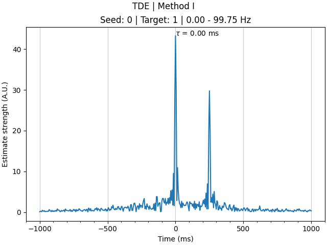
The estimated time delay without antisymmetrisation is 0 ms.
The estimated time delay with antisymmetrisation is 250 ms.

([<Figure size 640x480 with 1 Axes>], [array([<Axes: title={'center': 'Seed: 0 | Target: 1 | 0.00 - 99.75 Hz'}, xlabel='Time (ms)', ylabel='Estimate strength (A.U.)'>],
      dtype=object)])

References

[1]

Chrysostomos L. Nikias and Renlong Pan. Time delay estimation in unknown Gaussian spatially correlated noise. IEEE Transactions on Acoustics, Speech, and Signal Processing, 36(11):1706–1714, 1988. doi:10.1109/29.9008.

[2]

Federico Chella, Laura Marzetti, Vittorio Pizzella, Filippo Zappasodi, and Guido Nolte. Third order spectral analysis robust to mixing artifacts for mapping cross-frequency interactions in EEG/MEG. NeuroImage, 91:146–161, 2014. doi:10.1016/j.neuroimage.2013.12.064.

[3] (1,2)

Tin Jurhar and others. Estimating signal time-delays under mixed noise influence with novel cross- and bispectrum methods. In Preparation, In Preparation.