Compute time-resolved bispectral features

This example demonstrates how time-resolved bispectral features can be computed with PyBispectra.

# Author(s):
#   Thomas S. Binns | github.com/tsbinns

# sphinx_gallery_multi_image = "single"

import numpy as np
from matplotlib import pyplot as plt
from numpy.random import RandomState

from pybispectra import WaveShape, get_example_data_paths, compute_tfr

Background

Properties of signals can change over time within epochs/trials, for instance, according to changes in presented stimuli or task demands. In these cases, standard Fourier coefficients that aggregate frequency information across the entire duration of the epoch can be insufficient. In contrast, time-frequency representations (TFRs) offer a time-resolved view of frequency information, allowing us to analyse temporal dynamics of spectral features.

Just as Fourier coefficients can be used to compute bispectral features, so too can TFR coefficients, allowing for time-resolved bispectral analyses. In PyBispectra, time-resolved features can be computed from TFRs for:

• Phase-amplitude coupling: PAC

• Waveshape: WaveShape

• General analysis: Bispectrum and Threenorm

In this example, we will focus on the time-resolved analysis of waveshape features, however the same concept applies to all classes and analyses listed above.

Loading data and computing TFR coefficients

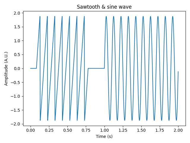
We will start by loading some example non-sinusoidal (sawtooth) data, simulated as a bursting oscillator at 10 Hz. We also simulate a corresponding sine wave at 10 Hz. Both signals consist of 1-second-long epochs which we concatenate along the time axis, such that the first second contains the sawtooth wave, and the final second the sine wave.

We compute the TFR coefficients of the concatenated data using the compute_tfr() function. By default, the TFR is constructed using Morlet wavelets, and the TFR amplitude returned. However, we require complex-valued TFR coefficients for the bispectral analysis, so we specify these to be returned with the output="complex" argument. We must also specify the frequencies we want to compute the TFR for, which we set here to 1-100 Hz.

# load example non-sinusoidal data
data_sawtooths = np.load(get_example_data_paths("sim_data_waveshape_sawtooths"))
data_sawtooths = data_sawtooths[:, [0], :]  # select ramp up sawtooth data
sampling_freq = 1000  # Hz
n_epochs, _, n_times = data_sawtooths.shape
times = np.linspace(0, (n_times / sampling_freq), n_times, endpoint=False)

# simulate sine wave data
data_sine = np.sin(2 * np.pi * 10 * times)
data_sine = np.repeat(data_sine[np.newaxis, np.newaxis, :], n_epochs, axis=0)
data_sine *= np.max(
    np.abs(data_sawtooths), axis=(1, 2), keepdims=True
)  # scale amplitude to match sawtooth data

# join sawtooth and sine data along time axis
data = np.concatenate((data_sawtooths, data_sine), axis=2)
n_times = data.shape[2]
times = np.linspace(0, (n_times / sampling_freq), n_times, endpoint=False)

# plot timeseries data
fig, axis = plt.subplots(1)
axis.plot(times, data[15, 0])
axis.set_title("Sawtooth & sine wave")
axis.set_xlabel("Time (s)")
axis.set_ylabel("Amplitude (A.U.)")
fig.tight_layout()

# add noise for numerical stability
random = RandomState(44)
snr = 0.25
data = snr * data + (1 - snr) * random.rand(*data.shape)

# compute TFR coeffs.
freqs = np.arange(1, 101)
tfr_coeffs, freqs = compute_tfr(
    data=data,
    sampling_freq=sampling_freq,
    freqs=freqs,
    n_cycles=freqs / 1.25,
    output="complex",
    verbose=False,
)

print(
    f"TFR coeffs.: [{tfr_coeffs.shape[0]} epochs x {tfr_coeffs.shape[1]} channel x "
    f"{tfr_coeffs.shape[2]} frequencies x {tfr_coeffs.shape[3]} timepoints]"
)

TFR coeffs.: [30 epochs x 1 channel x 100 frequencies x 2000 timepoints]

As you can see, the example epoch shows the sawtooth wave in the first second and the sine wave in the final second, and the TFR coefficients contain information on the frequency content of the data for each timepoint.

Computing time-resolved bispectral features

To compute waveshape, we start by initialising the WaveShape class object with the TFR coefficients, and the frequency and time information. To compute waveshape, we call the compute() method.

We specify the frequency arguments f1s and f2s to compute waveshape on in the range 5-35 Hz (around the frequency at which the signal features were simulated).

We can also specify the time period to compute waveshape on using the times argument. By default, the entire time period is taken, which we use here. A demonstration of specifying a subset of timepoints to compute features on is shown at the end of the example.

waveshape = WaveShape(
    data=tfr_coeffs,
    freqs=freqs,
    sampling_freq=sampling_freq,
    times=times,
    verbose=False,
)  # initialise object
waveshape.compute(
    f1s=(5, 35),
    f2s=(5, 35),
    times=None,  # compute features for all timepoints
)  # compute waveshape

# return results as an array
waveshape_results = waveshape.results.get_results(copy=False)

print(
    f"Waveshape results: [{waveshape_results.shape[0]} channel x "
    f"{waveshape_results.shape[1]} f1s x {waveshape_results.shape[2]} f2s x "
    f"{waveshape_results.shape[3]} timepoints]"
)

Waveshape results: [1 channel x 31 f1s x 31 f2s x 2000 timepoints]

We can see that waveshape features have been computed for the specified frequency combinations and all timepoints, averaged across our epochs.

Plotting time-resolved bispectral features

Let us now inspect the results. Information about the different waveshape features are encoded in different aspects of the complex-valued bicoherence. For a detailed explanation, see Compute waveshape features and Bartz et al. [1], but in brief, sawtooth waves are captured in the imaginary part. For our sawtooth wave simulated at 10 Hz, we expect the imaginary bicoherence values at this frequency and the higher harmonics (i.e., 20 and 30 Hz) to be non-zero. For the simulated sine wave, we do not expect non-zero bicoherence values at the simulated 10 Hz frequency, as the bispectrum selectively captures non-sinusoidal signal characteristics.

To demonstrate the time-resolved nature of the analysis, we will plot the results for two time periods: 0-1 seconds (containing the sawtooth wave); and 1-2 seconds (containing the sine wave). We specify these time periods using the times argument of the plot() method, which aggregates the time-resolved results by averaging over the selected timepoints.

figs, axes = waveshape.results.plot(
    times=(0, 1),  # time period to average over when plotting
    major_tick_intervals=10,
    minor_tick_intervals=2,
    cbar_range_abs=(0, 1),
    cbar_range_real=(0, 1),
    cbar_range_imag=(0, 1),
    cbar_range_phase=(0, 2),
    plot_absolute=True,
    show=False,
)
figs[0].suptitle("Sawtooth")
figs[0].set_size_inches(6, 6)
figs[0].show()

figs, axes = waveshape.results.plot(
    times=(1, 2),  # time period to average over when plotting
    major_tick_intervals=10,
    minor_tick_intervals=2,
    cbar_range_abs=(0, 1),
    cbar_range_real=(0, 1),
    cbar_range_imag=(0, 1),
    cbar_range_phase=(0, 2),
    plot_absolute=True,
    show=False,
)
figs[0].suptitle("Sine wave")
figs[0].set_size_inches(6, 6)
figs[0].show()

• 
• 

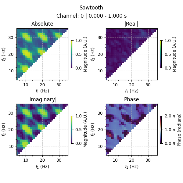
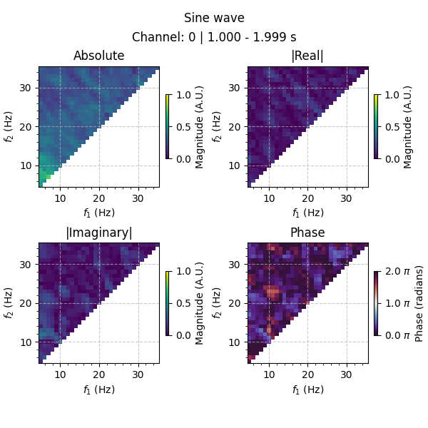
As expected, strong non-sinusoidal activity at 10 Hz and the harmonics is observed in the first second of the epochs (the time period of the sawtooth wave), with no strong non-sinusoidal activity in the final second (the time period of the sine wave).

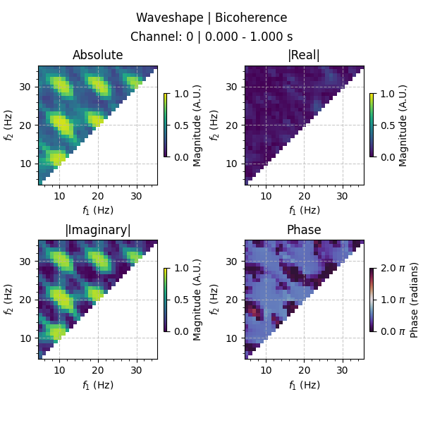
Specifying the time window to compute features on

As mentioned above, we can also specify a particular window to compute time-resolved features on. Here, we choose to only compute waveshape features for the first second of each epoch by specifying the times argument of the compute() method.

waveshape_0_1 = WaveShape(
    data=tfr_coeffs,
    freqs=freqs,
    sampling_freq=sampling_freq,
    times=times,
    verbose=False,
)  # initialise object
waveshape_0_1.compute(
    f1s=(5, 35),
    f2s=(5, 35),
    times=(0, 1),  # seconds
)

waveshape_results_0_1 = waveshape_0_1.results.get_results(copy=False)

print(
    f"Waveshape results: [{waveshape_results_0_1.shape[0]} channel x "
    f"{waveshape_results_0_1.shape[1]} f1s x {waveshape_results_0_1.shape[2]} f2s x "
    f"{waveshape_results_0_1.shape[3]} timepoints]"
)

figs, axes = waveshape_0_1.results.plot(
    times=None,  # use all available timepoints (0-1 s)
    major_tick_intervals=10,
    minor_tick_intervals=2,
    cbar_range_abs=(0, 1),
    cbar_range_real=(0, 1),
    cbar_range_imag=(0, 1),
    cbar_range_phase=(0, 2),
    plot_absolute=True,
    show=False,
)
figs[0].set_size_inches(6, 6)
figs[0].show()

Waveshape results: [1 channel x 31 f1s x 31 f2s x 1001 timepoints]

As we can see, the number of timepoints in the results is reduced accordingly, and the results visually match those plotted above for the first second of the data.

References

[1]

Sarah Bartz, Forooz Shahbazi Avarvand, Gregor Leicht, and Guido Nolte. Analyzing the waveshape of brain oscillations with bicoherence. NeuroImage, 188:145–160, 2019. doi:10.1016/j.neuroimage.2018.11.045.