Compute the bispectrum and threenorm

This example demonstrates how the bispectrum and threenorm can be computed.

# Author(s):
#   Thomas S. Binns | github.com/tsbinns

import numpy as np

from pybispectra import (
    compute_fft,
    get_example_data_paths,
    Bispectrum,
    PAC,
    ResultsCFC,
    Threenorm,
)

Background

The bispectrum can be used for various types of signal analysis, including phase-amplitude coupling [1], non-sinusoidal waveshape [2], and time delay estimation [3].

Although PyBispectra offers dedicated tools for computing these metrics, this involves taking information from specific combinations of channels (see: Compute phase-amplitude coupling; Compute waveshape features; and Compute time delay estimates).

For your analyses, you may wish to specify the combination of channels freely, a feature offered by Bispectrum (and the equivalent Threenorm for normalisation [4]).

In this example, we will demonstrate how these classes can be used to freely compute the bispectrum and threenorm, and show by comparing to the dedicated classes that the same information is captured in these general tools.

Here, we focus on phase-amplitude coupling (PAC). The bispectrum has the general form

\(\textbf{B}_{kmn}(f_1,f_2)=<\textbf{k}(f_1)\textbf{m}(f_2)\textbf{n}^* (f_2+f_1)>\) ,

where \(kmn\) is a combination of signals with Fourier coefficients \(\textbf{k}\), \(\textbf{m}\), and \(\textbf{n}\), respectively; and \(<>\) represents the average value over epochs. The computation of PAC follows from this [1]

\(\textbf{B}_{xyy}(f_1,f_2)=<\textbf{x}(f_1)\textbf{y}(f_2)\textbf{y}^* (f_2+f_1)>\) ,

\(\textrm{PAC}(\textbf{x}_{f_1},\textbf{y}_{f_2})=|\textbf{B}_{xyy}(f_1, f_2)|\) .

Computing PAC with the dedicated class

We start by computing PAC using the dedicated PAC class, which we will take as our reference for results.

The data we load here is simulated data containing coupling between the 10 Hz phase of one signal (index 0) and the 60 Hz amplitude of another (index 1).

# load simulated data
data = np.load(get_example_data_paths("sim_data_pac_bivariate"))
sampling_freq = 200  # sampling frequency in Hz

# compute Fourier coeffs.
fft_coeffs, freqs = compute_fft(
    data=data,
    sampling_freq=sampling_freq,
    n_points=sampling_freq,
    verbose=False,
)

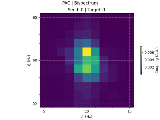
# compute & plot PAC
pac = PAC(
    data=fft_coeffs, freqs=freqs, sampling_freq=sampling_freq, verbose=False
)  # initialise object
pac.compute(indices=((0,), (1,)))  # compute PAC
pac_results = pac.results.get_results()  # extract results array
pac.results.plot(f1s=(5, 15), f2s=(55, 65))  # plot PAC

([<Figure size 640x480 with 2 Axes>], [array([<Axes: title={'center': 'Seed: 0 | Target: 1'}, xlabel='$f_1$ (Hz)', ylabel='$f_2$ (Hz)'>],
      dtype=object)])

As expected, we observe 10-60 Hz PAC with channel index 0 as our seed (\(x\); 10 Hz phase) and channel index 1 as our target (\(y\); 60 Hz amplitude).

With the dedicated PAC class, the seeds and targets are automatically assigned to the appropriate \(kmn\) combination when computing the bispectrum, in this case \(xyy\).

Computing PAC with the general class

However, an equivalent result can be obtained using the Bispectrum class and specifying the combination of \(kmn=xyy\) manually.

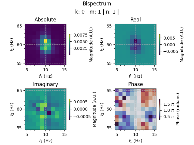
# compute the bispectrum where kmn = xyy & plot results
bs = Bispectrum(
    data=fft_coeffs, freqs=freqs, sampling_freq=sampling_freq, verbose=False
)  # initialise object
bs.compute(indices=((0,), (1,), (1,)))  # kmn = xyy
bs.results.plot(f1s=(5, 15), f2s=(55, 65))  # plot bispectrum

([<Figure size 640x480 with 8 Axes>], [array([[<Axes: title={'center': 'Absolute'}, xlabel='$f_1$ (Hz)', ylabel='$f_2$ (Hz)'>,
        <Axes: title={'center': 'Real'}, xlabel='$f_1$ (Hz)', ylabel='$f_2$ (Hz)'>,
        <Axes: title={'center': 'Imaginary'}, xlabel='$f_1$ (Hz)', ylabel='$f_2$ (Hz)'>,
        <Axes: title={'center': 'Phase'}, xlabel='$f_1$ (Hz)', ylabel='$f_2$ (Hz)'>]],
      dtype=object)])

Since the bispectrum is complex-valued, we must take the absolute value to compare to PAC. Additionally, we can package the results into the dedicated ResultsCFC class for cross-frequency coupling results.

Plotting the results alongside each other shows they are identical.

# package general class results
bs_pac = ResultsCFC(
    data=np.abs(bs.results.get_results()),
    indices=((0,), (1,)),
    f1s=bs.results.f1s,
    f2s=bs.results.f2s,
    name="PAC | Bispectrum (manual)",
)
bs_pac_results = bs_pac.get_results()

# compare general and dedicated class results
if np.all(
    bs_pac_results[~np.isnan(bs_pac_results)]
    == pac_results[~np.isnan(pac_results)]
):
    print("Results are identical!")
else:
    print("Results are not identical!")

pac.results.plot(f1s=(5, 15), f2s=(55, 65))  # dedicated class
bs_pac.plot(f1s=(5, 15), f2s=(55, 65))  # general class

• 
• 

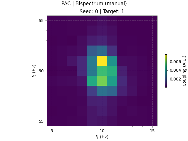
Results are identical!

([<Figure size 640x480 with 2 Axes>], [array([<Axes: title={'center': 'Seed: 0 | Target: 1'}, xlabel='$f_1$ (Hz)', ylabel='$f_2$ (Hz)'>],
      dtype=object)])

Bispectrum normalisation

The bispectrum can also be normalised to the bicoherence, \(\boldsymbol{\mathcal{B}}\), using the threenorm, \(\textbf{N}\), [4]

\(\textbf{N}_{xyy}(f_1,f_2)=(<|\textbf{x}(f_1)|^3><|\textbf{y}(f_2)|^3> <|\textbf{y}(f_2+f_1)|^3>)^{\frac{1}{3}}\) ,

\(\boldsymbol{\mathcal{B}}_{xyy}(f_1,f_2)=\Large\frac{\textbf{B}_{xyy} (f_1,f_2)}{\textbf{N}_{xyy}(f_1,f_2)}\) ,

where the resulting values lie in the range \([-1, 1]\), controlling for the amplitude of the signals.

While the dedicated PAC class has an option for performing this normalisation, we can also compute the threenorm separately using the Threenorm class and apply the normalisation manually.

Again, we specify the \(kmn\) channel combination as \(xyy\) for our seed (\(x\)) and target (\(y\)).

# compute the threenorm
norm = Threenorm(
    data=fft_coeffs, freqs=freqs, sampling_freq=sampling_freq, verbose=False
)  # initialise object
norm.compute(indices=((0,), (1,), (1,)))  # kmn = xyy

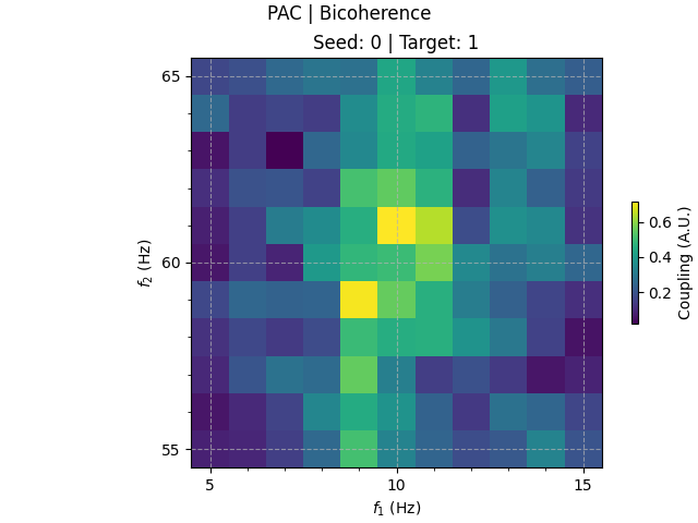
# normalise the bispectrum
bicoh = np.abs(bs.results.get_results() / norm.results.get_results())

# package bicoherence results
bicoh_pac = ResultsCFC(
    data=bicoh,
    indices=((0,), (1,)),
    f1s=bs.results.f1s,
    f2s=bs.results.f2s,
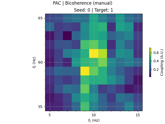
    name="PAC | Bicoherence (manual)",
)
bicoh_pac_results = bicoh_pac.get_results()

Comparing these bicoherence values with those obtained from the dedicated PAC class, we see that both approaches produce identical results.

# compute bicoherence PAC with dedicated class
pac_norm = PAC(
    data=fft_coeffs, freqs=freqs, sampling_freq=sampling_freq, verbose=False
)  # initialise object
pac_norm.compute(indices=((0,), (1,)), norm=True)  # compute PAC
pac_norm_results = pac_norm.results.get_results()  # extract results array

# compare general and dedicated class results
if np.all(
    bicoh_pac_results[~np.isnan(bicoh_pac_results)]
    == pac_norm_results[~np.isnan(pac_norm_results)]
):
    print("Results are identical!")
else:
    print("Results are not identical!")

pac_norm.results.plot(f1s=(5, 15), f2s=(55, 65))  # dedicated class
bicoh_pac.plot(f1s=(5, 15), f2s=(55, 65))  # general class

• 
• 

Results are identical!

([<Figure size 640x480 with 2 Axes>], [array([<Axes: title={'center': 'Seed: 0 | Target: 1'}, xlabel='$f_1$ (Hz)', ylabel='$f_2$ (Hz)'>],
      dtype=object)])

Manual computation of waveshape results and antisymmetrisation

The Bispectrum and Threenorm classes can also be used to compute non-sinusoidal waveshape results (equivalent to WaveShape) and antisymmetrised bispectra (e.g. as in PAC) by following the equations listed in the respective documentation and publications.

Conclusion

Altogether, the Bispectrum and Threenorm classes provide a flexible way to compute bispectra and normalisation terms with custom \(kmn\) channel combinations.

References

[1] (1,2)

Christopher K. Kovach, Hiroyuki Oya, and Hiroto Kawasaki. The bispectrum and its relationship to phase-amplitude coupling. NeuroImage, 173:518–539, 2018. doi:10.1016/j.neuroimage.2018.02.033.

[2]

Sarah Bartz, Forooz Shahbazi Avarvand, Gregor Leicht, and Guido Nolte. Analyzing the waveshape of brain oscillations with bicoherence. NeuroImage, 188:145–160, 2019. doi:10.1016/j.neuroimage.2018.11.045.

[3]

Chrysostomos L. Nikias and Renlong Pan. Time delay estimation in unknown Gaussian spatially correlated noise. IEEE Transactions on Acoustics, Speech, and Signal Processing, 36(11):1706–1714, 1988. doi:10.1109/29.9008.

[4] (1,2)

Forooz Shahbazi, Arne Ewald, and Guido Nolte. Univariate normalization of bispectrum using Hölder’s inequality. Journal of Neuroscience Methods, 233:177–186, 2014. doi:10.1016/j.jneumeth.2014.05.030.