Spatio-spectral filtering for waveshape analysis

This example demonstrates how spatio-spectral filtering can be incorporated into waveshape analysis with PyBispectra.

# Author(s):
#   Thomas S. Binns | github.com/tsbinns

import numpy as np

from pybispectra import (
    compute_fft,
    compute_rank,
    get_example_data_paths,
    SpatioSpectralFilter,
    WaveShape,
    ResultsWaveShape,
)

Background

When analysing signals, important information may be gleaned from a variety of features, including their shape. One tool for extracting this information is the bicoherence, capturing information about rise-decay asymmetry (i.e. how much a signal resembles a sawtooth wave) and peak-trough asymmetry (i.e. how ‘spiky’ a signal is) [1]. The use of the bicoherence for waveshape analysis was discussed in detail in this example: Compute waveshape features. In particular, it was mentioned how the signal-to-noise ratio of the signal can affect the ability of the bicoherence to extract information about waveshape. In this example, we will look at how spatio-spectral filtering can be used to improve the SNR of signals and enhance waveshape analyses.

Loading data and performing spatio-spectral filtering

We will start by loading some example data. This data consists of a peak-dominant, ramp down sawtooth bursting oscillator simulated at 20 Hz, and combined with a mixture of 20 independent pink noise sources for a signal-to-noise ratio of 0.1. This setup therefore reflects a typical electrophysiolgical recording scenario where the brain source of interest projects to multiple sensors and is combined with multiple noise sources.

Two forms of spatio-spectral filtering are available in PyBispectra: spatio-spectral decomposition (SSD) [2]; and harmonic power maximisation (HPMax) [1]. Both methods are based on generalised eigendecompositions [3]. In SSD, a frequency band of interest is chosen as the signal, and the flanking frequencies are designated as the noise. The data is filtered in these signal and noise ranges, and the covariance matrices of the corresponding data are used to generate a set of spatial filters that, when applied to the data, maximise the SNR (i.e. maximise signal power at the desired frequency band). HPMax can be thought of as an extension of SSD, in which the base frequency band and its higher harmonics are designated as the signal, based on the principle that non-sinusoidal signal information is encoded at its base frequency and higher harmonics.

The ability of SSD and HPMax to recover information about the underlying wave shape of a signal of interest varies depending on the SNR of the data and the colour of the noise [1]. At an SNR of 0.1 with pink noise, both SSD and HPMax are able to recover waveshape information well, however for simplicity we will focus only one: HPMax.

To perform spatio-spectral filtering, we start by initialising the SpatioSpectralFilter class object with the data and the sampling frequency. To compute HPMax, we call the fit_transform_hpmax() method (SSD can be computed using the fit_transform_ssd() method). We specify the ‘signal’ frequency band of interest to be 18-22 Hz and the flanking ‘noise’ frequencies to be 15-18 Hz and 22-25 Hz. Additionally, we take information from the two higher harmonics of the ‘signal’ frequencies (i.e. 36-44 Hz and 54-66 Hz).

After finding the filters, we use them to transform the data. By default, only those filters whose signal vs. noise contributions are greater than 1 are returned, however for simplicity we will take only the first component (i.e. the component with the greatest signal-to-noise ratio).

# load example data
data = np.load(get_example_data_paths("sim_data_waveshape_noisy"))
sampling_freq = 1000  # Hz

# perform spatio-spectral filtering
ssf = SpatioSpectralFilter(
    data=data, sampling_freq=sampling_freq, verbose=False
)
ssf.fit_transform_hpmax(
    signal_bounds=(18, 22), noise_bounds=(15, 25), n_harmonics=2
)

# return the first component of the filtered data
transformed_data = (ssf.get_transformed_data()[:, 0])[:, np.newaxis, :]

print(
    f"Original timeseries data: [{data.shape[0]} epochs x {data.shape[1]} "
    f"channel(s) x {data.shape[2]} times]"
)
print(
    f"Transformed timeseries data: [{transformed_data.shape[0]} epochs x "
    f"{transformed_data.shape[1]} channel(s) x {transformed_data.shape[2]} "
    "times]\nSignal-to-noise ratio of transformed data's first component: "
    f"{ssf.ratios[0] :.2f}"
)

Original timeseries data: [30 epochs x 20 channel(s) x 1000 times]
Transformed timeseries data: [30 epochs x 1 channel(s) x 1000 times]
Signal-to-noise ratio of transformed data's first component: 16.14

As SSD and HPMax are based on generalised eigendecomposition, the data for which the filters are being generated must be full rank (i.e. a non-zero determinant). The fit_transform_ssd() and fit_transform_hpmax() methods have a rank argument where the rank of the data can be specified, according to which the data will be projected to. If the rank is not specified, it will be computed automatically using the compute_rank() function. Here, the rank is determined based on the number of non-zero singular values. Non-zero singular values are defined as those which are greater than the largest singular value multiplied by a tolerance value specified by the sv_tol argument (\(1e^{-5}\) by default).

Below we see that our original timeseries data of 20 channels has a rank of 20, and is therefore full rank. Although the rank of the data is automatically computed, the option of specifying the rank subspace to project the data to is still provided, as a rank projection less than that of the data’s rank may be desired when dealing with a large number of channels to prevent the overfitting of filters.

rank = compute_rank(data, sv_tol=1e-5)
print(
    f"The original timeseries data ({data.shape[1]} channels) has a rank of "
    f"{rank}."
)

The original timeseries data (20 channels) has a rank of 20.

Computing and plotting waveshape features

For the waveshape analysis, we compute the Fourier coefficients of the data and use them to initialise the WaveShape class object. To compute waveshape, we call the compute() method.

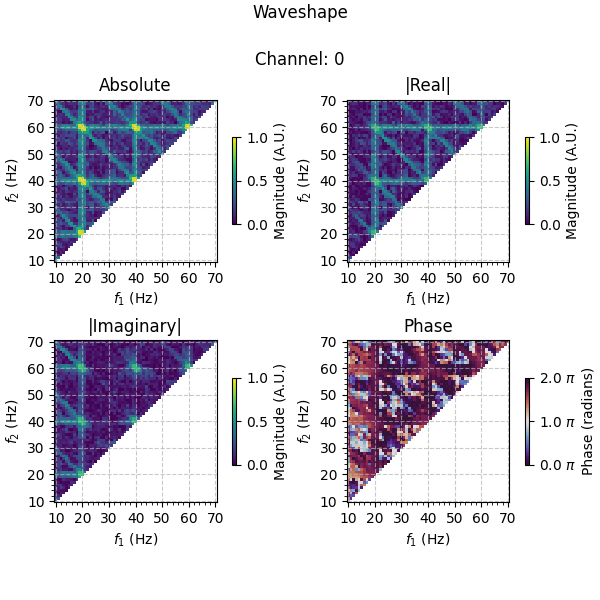
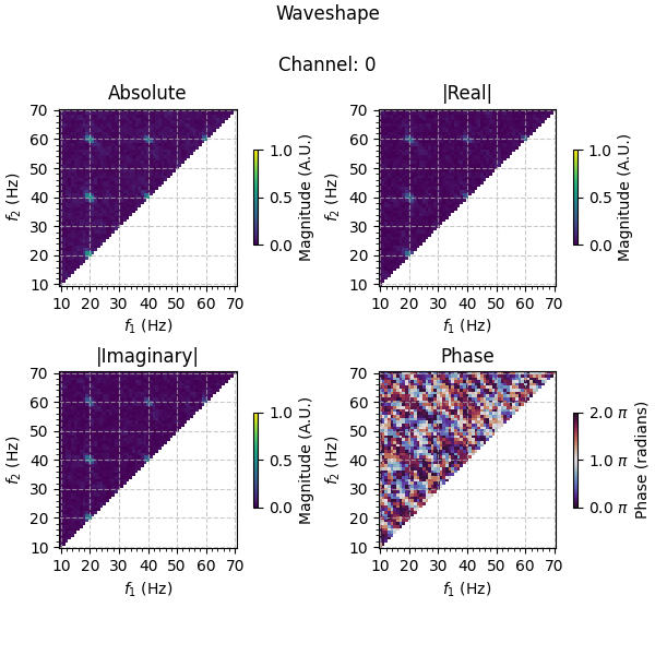
Plotting the results, we see that information is captured in both the real and imaginary part of the bicoherence at 20 Hz and its higher harmonics, as we expect given that the simulated source consists of both peak-trough and rise-decay asymmetries. Looking at the phases, we see that the results are ~ \(\frac{7}{4}\pi\) at these frequencies, in line with the fact that the simulated source is a peak-dominant (positive real-value), ramp down (negative imaginary-value) wave. Comparing to the results of the unfiltered data averaged over channels, the waveshape information is much clearer in the filtered data.

# transformed data
fft_coeffs_transformed, freqs = compute_fft(
    data=transformed_data,
    sampling_freq=sampling_freq,
    n_points=sampling_freq,
    verbose=False,
)
waveshape_transformed = WaveShape(
    data=fft_coeffs_transformed,
    freqs=freqs,
    sampling_freq=sampling_freq,
    verbose=False,
)
waveshape_transformed.compute(f1s=(10, 70), f2s=(10, 70))
fig, axes = waveshape_transformed.results.plot(
    major_tick_intervals=10,
    minor_tick_intervals=2,
    cbar_range_abs=(0, 1),
    cbar_range_real=(0, 1),
    cbar_range_imag=(0, 1),
    cbar_range_phase=(0, 2),
    plot_absolute=True,
)
fig[0].set_size_inches(6, 6)

# noisy data
fft_coeffs_noisy, freqs = compute_fft(
    data=data,
    sampling_freq=sampling_freq,
    n_points=sampling_freq,
    verbose=False,
)
waveshape_noisy = WaveShape(
    data=fft_coeffs_noisy,
    freqs=freqs,
    sampling_freq=sampling_freq,
    verbose=False,
)
waveshape_noisy.compute(f1s=(10, 70), f2s=(10, 70))
noisy_results = waveshape_noisy.results.get_results()
noisy_results = noisy_results.mean(axis=0)[np.newaxis, :, :]
noisy_results = ResultsWaveShape(
    data=noisy_results,
    indices=(0,),
    f1s=waveshape_noisy.results.f1s,
    f2s=waveshape_noisy.results.f2s,
    name=waveshape_noisy.results.name,
)
fig, axes = noisy_results.plot(
    major_tick_intervals=10,
    minor_tick_intervals=2,
    cbar_range_abs=(0, 1),
    cbar_range_real=(0, 1),
    cbar_range_imag=(0, 1),
    cbar_range_phase=(0, 2),
    plot_absolute=True,
)
fig[0].set_size_inches(6, 6)

• 
• 

As you can see, spatio-spectral filtering is a powerful tool for extracting waveshape information from noisy data, and the tools in PyBispectra allow you to easily incorporate these methods into your analysis pipeline.

References

[1] (1,2,3)

Sarah Bartz, Forooz Shahbazi Avarvand, Gregor Leicht, and Guido Nolte. Analyzing the waveshape of brain oscillations with bicoherence. NeuroImage, 188:145–160, 2019. doi:10.1016/j.neuroimage.2018.11.045.

[2]

Vadim V. Nikulin, Guido Nolte, and Gabriel Curio. A novel method for reliable and fast extraction of neuronal EEG/MEG oscillations on the basis of spatio-spectral decomposition. NeuroImage, 55(4):1528–1535, 2011. doi:10.1016/j.neuroimage.2011.01.057.

[3]

Michael X. Cohen. A tutorial on generalized eigendecomposition for denoising, contrast enhancement, and dimension reduction in multichannel electrophysiology. Neuroimage, 247:118809, 2022. doi:10.1016/j.neuroimage.2021.118809.