Compute waveshape features

This example demonstrates how waveshape features can be computed with PyBispectra.

# Author(s):
#   Thomas S. Binns | github.com/tsbinns

import numpy as np
from numpy.random import RandomState
from matplotlib import pyplot as plt

from pybispectra import compute_fft, get_example_data_paths, WaveShape

Background

When analysing signals, important information may be gleaned from a variety of features, including their shape. For example, in neuroscience it has been suggested that non-sinusoidal waves may play important roles in physiology and pathology, such as waveform sharpness reflecting synchrony of synaptic inputs [1] and correlating with symptoms of Parkinson’s disease [2]. Two aspects of waveshape described in recent literature include: rise-decay asymmetry - how much the wave resembles a sawtooth pattern (also called waveform sharpness or derivative skewness); and peak-trough asymmetry - whether peaks (events with a positive-valued amplitude) or troughs (events with a negative-valued amplitude) are more dominant in the signal (also called signal/value skewness).

A common strategy for waveshape analysis involves identifying and characterising the features of waves in time-series data - see Cole et al. (2017) [2] for an example. Naturally, it can be of interest to explore the shapes of signals at particular frequencies, in which case the time-series data can be bandpass filtered. There is, however, a major limitation to this approach: applying a bandpass filter to data can seriously alter non-sinusoidal signal shape, compromising any analysis of waveshape before it has begun.

Thankfully, the bispectrum captures information about non-sinudoisal waveshape, enabling spectrally-resolved analyses at a fine frequency resolution without the need for bandpass filtering. In particular, the bispectrum contains information about rise-decay asymmetry (encoded in the imaginary part of the bispectrum) and peak-trough asymmetry (encoded in the real part of the bispectrum) [3].

The bispectrum has the general form

\(\textbf{B}_{kmn}(f_1,f_2)=<\textbf{k}(f_1)\textbf{m}(f_2)\textbf{n}^* (f_2+f_1)>\) ,

where \(kmn\) is a combination of signals with Fourier coefficients \(\textbf{k}\), \(\textbf{m}\), and \(\textbf{n}\), respectively; \(f_1\) and \(f_2\) correspond to a lower and higher frequency, respectively; and \(<>\) represents the average value over epochs. When analysing waveshape, we are interested in only a single signal, and as such \(k=m=n\).

Furthermore, we can normalise the bispectrum to the bicoherence, \(\boldsymbol{\mathcal{B}}\), using the threenorm, \(\textbf{N}\), [4]

\(\textbf{N}_{xxx}(f_1,f_2)=(<|\textbf{x}(f_1)|^3><|\textbf{x}(f_2)|^3> <|\textbf{x}(f_2+f_1)|^3>)^{\frac{1}{3}}\) ,

\(\boldsymbol{\mathcal{B}}_{xxx}(f_1,f_2)=\Large\frac{\textbf{B}_{xxx} (f_1,f_2)}{\textbf{N}_{xxx}(f_1,f_2)}\) ,

where the resulting values lie in the range \([-1, 1]\).

Loading data and computing Fourier coefficients

We will start by loading some example data and computing the Fourier coefficients using the compute_fft() function. This data consists of sawtooth waves (information will be captured in the rise-decay asymmetry) and waves with a dominance of peaks or troughs (information will be captured in the peak-trough asymmetry), all simulated as bursting oscillators at 10 Hz.

# load example data
data_sawtooths = np.load(
    get_example_data_paths("sim_data_waveshape_sawtooths")
)
data_peaks_troughs = np.load(
    get_example_data_paths("sim_data_waveshape_peaks_troughs")
)
sampling_freq = 1000  # Hz

# plot timeseries data
times = np.linspace(
    0, (data_sawtooths.shape[2] / sampling_freq), data_sawtooths.shape[2]
)
fig, axes = plt.subplots(2, 2)
axes[0, 0].plot(times, data_sawtooths[15, 0])
axes[0, 1].plot(times, data_sawtooths[15, 1])
axes[1, 0].plot(times, data_peaks_troughs[15, 0])
axes[1, 1].plot(times, data_peaks_troughs[15, 1])
titles = [
    "Ramp up sawtooth",
    "Ramp down sawtooth",
    "Peak dominance",
    "Trough dominance",
]
for ax, title in zip(axes.flatten(), titles):
    ax.set_title(title)
    ax.set_xlabel("Time (s)")
    ax.set_ylabel("Amplitude (A.U.)")
fig.tight_layout()

# add noise for numerical stability
random = RandomState(44)
snr = 0.25
datasets = [data_sawtooths, data_peaks_troughs]
for data_idx, data in enumerate(datasets):
    datasets[data_idx] = snr * data + (1 - snr) * random.rand(*data.shape)
data_sawtooths = datasets[0]
data_peaks_troughs = datasets[1]

# compute Fourier coeffs.
fft_coeffs_sawtooths, freqs = compute_fft(
    data=data_sawtooths,
    sampling_freq=sampling_freq,
    n_points=sampling_freq,
    verbose=False,
)
fft_coeffs_peaks_troughs, _ = compute_fft(
    data=data_peaks_troughs,
    sampling_freq=sampling_freq,
    n_points=sampling_freq,
    verbose=False,
)

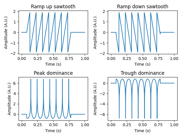
Plotting the data, we see that the sawtooth waves consist of a signal where the decay steepness is greater than the rise steepness (ramp up sawtooth) and a signal where the rise steepness is greater than the decay steepness (ramp down sawtooth). Additionally, the peak and trough waves consist of a signal where peaks are most dominant, and a signal where troughs are most dominant. After loading the data, we add some noise for numerical stability.

Computing waveshape features

To compute waveshape, we start by initialising the WaveShape class object with the Fourier coefficients and the frequency information. To compute waveshape, we call the compute() method. By default, waveshape is computed for all channels and all frequency combinations, however we can also specify particular channels and combinations of interest.

Here, we specify the frequency arguments f1s and f2s to compute waveshape on in the range 5-35 Hz (around the frequency at which the signal features were simulated). By leaving the indices argument blank, we will look at all channels in the data.

# sawtooth waves
waveshape_sawtooths = WaveShape(
    data=fft_coeffs_sawtooths,
    freqs=freqs,
    sampling_freq=sampling_freq,
    verbose=False,
)  # initialise object
waveshape_sawtooths.compute(f1s=(5, 35), f2s=(5, 35))  # compute waveshape

# peaks and troughs
waveshape_peaks_troughs = WaveShape(
    data=fft_coeffs_peaks_troughs,
    freqs=freqs,
    sampling_freq=sampling_freq,
    verbose=False,
)
waveshape_peaks_troughs.compute(f1s=(5, 35), f2s=(5, 35))  # compute waveshape

# return results as an array
waveshape_results = waveshape_sawtooths.results.get_results()

print(
    f"Waveshape results: [{waveshape_results.shape[0]} channels x "
    f"{waveshape_results.shape[1]} f1s x {waveshape_results.shape[2]} f2s]"
)

Waveshape results: [2 channels x 31 f1s x 31 f2s]

We can see that waveshape features have been computed for both channels and the specified frequency combinations, averaged across our epochs. Given the nature of the bispectrum, entries where \(f_1\) would be higher than \(f_2\), as well as where \(f_2 + f_1\) exceeds the frequency bounds of our data, cannot be computed. In such cases, the values corresponding to those ‘bad’ frequency combinations are numpy.nan.

Plotting waveshape features

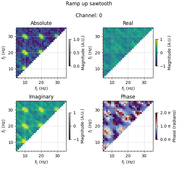
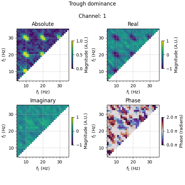
Let us now inspect the results. Information about the different waveshape features are encoded in different aspects of the complex-valued bicoherence, with peak-trough asymmetry encoded in the real part, and rise-decay asymmetry encoded in the imaginary part. We can therefore additionally examine the absolute value of the bicoherence (i.e. the magnitude) as well as the phase angle to get an overall picture of the combination of peak-trough and rise-decay asymmetries.

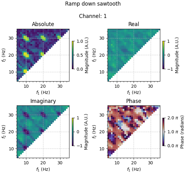
For the sawtooth waves, we expect the real part of bicoherence to be ~0 and the imaginary part to be non-zero at the simulated 10 Hz frequency. From the plots, we see that this is indeed the case. However, we also see that the imaginary values at the 10 Hz higher harmonics (i.e. 20 and 30 Hz) are also non-zero, a product of the Fourier transform’s application to non-sinusoidal signals. It is also worth noting that the sign of the imaginary values varies for the particular sawtooth type, with a ramp up sawtooth resulting in positive values, and a ramp down sawtooth resulting in negative values.

Information about the direction of the asymmetry is encoded not only in the sign of the bicoherence values, but also in its phase. As in Bartz et al. [3], we represent phase in the range \((0, 2\pi]\) (travelling counter-clockwise from the positive real axis). Accordingly, a phase of \(\frac{1}{2}\pi\) is seen at 10 Hz and its higher harmonics for the ramp up sawtooth, with a phase of \(\frac{3}{2}\pi\) for the ramp down sawtooth. The phases and absolute values (i.e. the magnitude) therefore combine information from both the real and imaginary components.

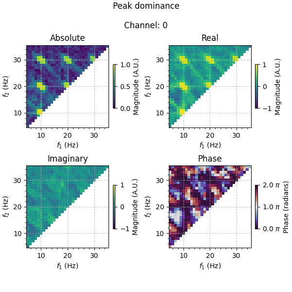
In contrast, we expect the real part of the bicoherence to be non-zero for signals with peak-trough asymmetry, and the imaginary part to be ~0. Again, this is what we observe. Similarly to before, the signs of the real values are positive for the peak-dominant signal, and negative for the trough-dominant signal, which is also reflected in the phases (~0 or 2 \(\pi\) for the peak-dominant signal, and \(\pi\) for the trough-dominant signal).

Here, we plotted the real and imaginary parts of the bicoherence without taking the absolute value. If the particular direction of asymmetry is not of interest, the absolute values can be plotted instead (by setting plot_absolute=True) to show the overall degree of asymmetry. In any case, the direction of asymmetry can be inferred from the phases.

Finally, note that the Figure and Axes objects can also be returned for any desired manual adjustments of the plots.

figs, axes = waveshape_sawtooths.results.plot(
    major_tick_intervals=10,
    minor_tick_intervals=2,
    cbar_range_abs=(0, 1),
    cbar_range_real=(-1, 1),
    cbar_range_imag=(-1, 1),
    cbar_range_phase=(0, 2),
    plot_absolute=False,
    show=False,
)
titles = ["Ramp up", "Ramp down"]
for fig, title in zip(figs, titles):
    fig.suptitle(f"{title} sawtooth")
    fig.set_size_inches(6, 6)
    fig.show()

figs, axes = waveshape_peaks_troughs.results.plot(
    major_tick_intervals=10,
    minor_tick_intervals=2,
    cbar_range_abs=(0, 1),
    cbar_range_real=(-1, 1),
    cbar_range_imag=(-1, 1),
    cbar_range_phase=(0, 2),
    plot_absolute=False,
    show=False,
)
titles = ["Peak", "Trough"]
for fig, title in zip(figs, titles):
    fig.suptitle(f"{title} dominance")
    fig.set_size_inches(6, 6)
    fig.show()

• 
• 
• 
• 

Analysing waveshape in low signal-to-noise ratio data

Depending on the degree of signal-to-noise ratio as well as the colour of the noise, the ability of the bispectrum to extract information about the underlying waveshape features can vary. To alleviate this, Bartz et al. [3] propose utilising spatio-spectral filtering to enhance the signal-to-noise ratio of the data at a frequency band of interest (which has the added benefit of enabling multivariate signal analysis). Details of how spatio-spectral filtering can be incorporated into waveshape analysis are presented in the following example: Spatio-spectral filtering for waveshape analysis.

References

[1]

Maxwell A. Sherman, Shane Lee, Robert Law, Saskia Haegens, Catherine A. Thorn, Matti S. Hämäläinen, Christopher I. Moore, and Stephanie R. Jones. Neural mechanisms of transient neocortical beta rhythms: Converging evidence from humans, computational modeling, monkeys, and mice. Proceedings of the National Academy of Sciences, 113(33):E4885–E4894, 2016. doi:10.1073/pnas.1604135113.

[2] (1,2)

Scott R. Cole, Roemer van der Meij, Erik J. Peterson, Coralie de Hemptinne, Philip A. Starr, and Bradley Voytek. Nonsinusoidal beta oscillations reflect cortical pathophysiology in Parkinson’s disease. Journal of Neuroscience, 37(18):4830–4840, 2017. doi:10.1523/JNEUROSCI.2208-16.2017.

[3] (1,2,3)

Sarah Bartz, Forooz Shahbazi Avarvand, Gregor Leicht, and Guido Nolte. Analyzing the waveshape of brain oscillations with bicoherence. NeuroImage, 188:145–160, 2019. doi:10.1016/j.neuroimage.2018.11.045.

[4]

Forooz Shahbazi, Arne Ewald, and Guido Nolte. Univariate normalization of bispectrum using Hölder’s inequality. Journal of Neuroscience Methods, 233:177–186, 2014. doi:10.1016/j.jneumeth.2014.05.030.