Compute time delay estimates for frequency bands

This example demonstrates how time delay estimation (TDE) for different frequency bands can be computed with PyBispectra.

# Author(s):
#   Thomas S. Binns | github.com/tsbinns

import numpy as np

from pybispectra import compute_fft, get_example_data_paths, TDE

Background

In the previous example, we looked at how the bispectrum can be used to compute time delays. In this example, we will take things further to look at how time delays can be computed for particular frequency bands. This can be of interest when two signals consist of multiple interacting sources at distinct frequency bands.

For example, in the brain, information flows from the motor cortex to the subthalamic nucleus of the subcortical basal ganglia via two distinct pathways: the monosynaptic hyperdirect pathway; and the polysynaptic indirect pathway. As such, cortico-subthalamic communication is faster via the hyperdirect pathway than via the indirect pathway [1]. Furthermore, hyperdirect and indirect pathway information flow is thought to be characterised by activity in higher (~20-30 Hz) and lower (~10-20 Hz) frequency bands, respectively. Accordingly, estimating time delays for these frequency bands could be used as a proxy for investigating information flow in these different pathways.

One approach for isolating frequency band information is to bandpass filter the data before computing time delays. However, this approach can fail to reveal the time true underlying time delay, even if the signals have a fairly high signal-to-noise ratio. In contrast, as the bispectrum is frequency-resolved, we can extract information for particular frequencies directly, with improved performance for revealing the true time delay.

Computing frequency band-resolved time delays

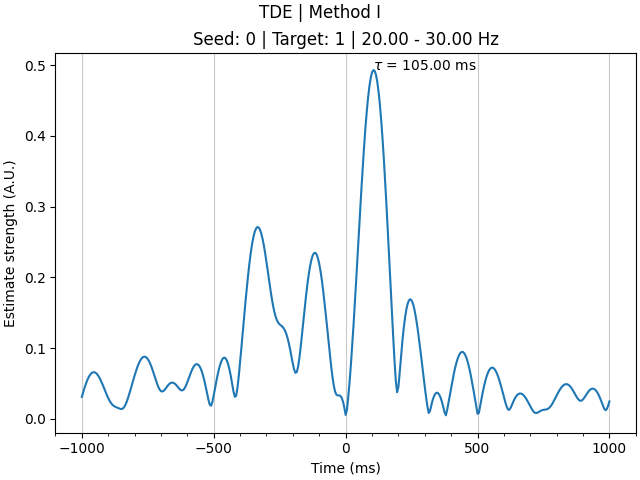
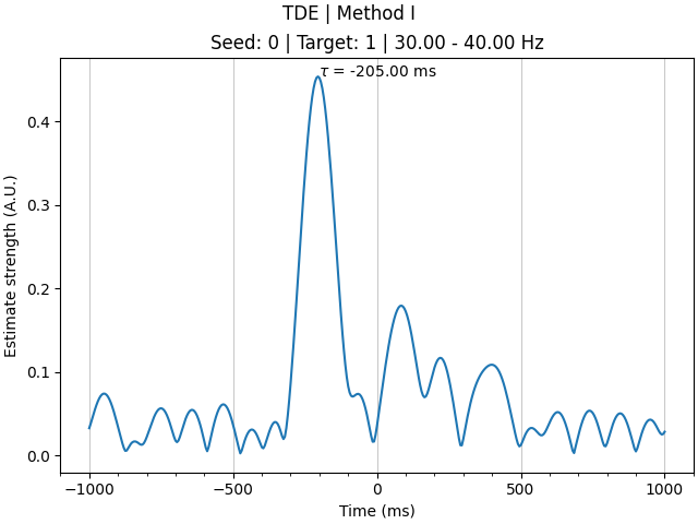
We will start by loading some simulated data consisting of two signals, \(\textbf{x}\) and \(\textbf{y}\). In these signals, there is delay of 100 ms from \(\textbf{x}\) to \(\textbf{y}\) in the 20-30 Hz range, and a delay of 200 ms from \(\textbf{y}\) to \(\textbf{x}\) in the 30-40 Hz range. As before, we compute the Fourier coefficients of the data, setting n_points to be twice the number of time points in each epoch of the data, plus one.

When computing time delay estimation, we extract information for the broadband spectrum, 20-30 Hz band, and 30-40 Hz band, using the fmin and fmax arguments.

# load simulated data
data = np.load(get_example_data_paths("sim_data_tde_fbands"))
sampling_freq = 200  # sampling frequency in Hz
n_times = data.shape[2]  # number of timepoints in the data

# compute Fourier coeffs.
fft_coeffs, freqs = compute_fft(
    data=data,
    sampling_freq=sampling_freq,
    n_points=2 * n_times + 1,  # recommended for time delay estimation
    window="hamming",
    verbose=False,
)

tde = TDE(
    data=fft_coeffs, freqs=freqs, sampling_freq=sampling_freq, verbose=False
)
tde.compute(indices=((0,), (1,)), fmin=(0, 20, 30), fmax=(100, 30, 40))

print(
    f"TDE results: [{tde.results.shape[0]} connections x "
    f"{tde.results.shape[1]} frequency bands x {tde.results.shape[2]} times]"
)

TDE results: [1 connections x 3 frequency bands x 401 times]

We can see that time delays have been computed for one connection (0 -> 1) and three frequency bands (0-100 Hz; 20-30 Hz; and 30-40 Hz), with 401 timepoints. The timepoints correspond to time delay estimates for every 5 ms (i.e. the sampling rate of the data), ranging from -1000 ms to +1000 ms.

Inspecting the results, we see that: the 20-30 Hz bispectrum entries capture the corresponding delay around 100 ms from \(\textbf{x}\) to \(\textbf{y}\); the 30-40 Hz bispectrum entries capture the delay around 200 ms from \(\textbf{y}\) to \(\textbf{x}\) (represented as a negative time delay from \(\textbf{x}\) to \(\textbf{y}\)); and the broadband 0-100 Hz bispectrum captures both frequency band interactions. As an additional note, you can see that computing time delays on smaller frequency bands (i.e. fewer Fourier coefficients) increases the temporal smoothing of results, something you must keep in mind if you expect your data to contain distinct interactions which are temporally proximal to one another.

fig, axes = tde.results.plot(freq_bands=(1, 2, 0))

• 
• 
• 

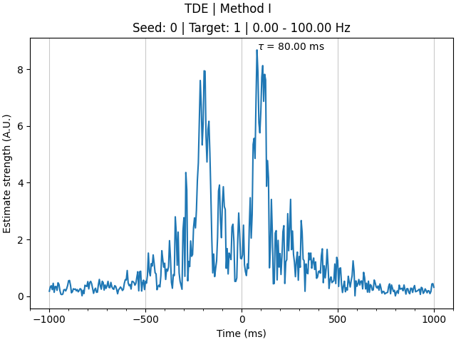
Altogether, estimating time delays for particular frequency bands is a useful approach to discriminate interactions between signals at distinct frequencies, whether these frequency bands come from an a priori knowledge of the system being studied (e.g. as for cortico-subthalamic interactions), or after observing multiple peaks in the broadband time delay spectrum.

References

[1]

Zlata Polyakova, Satomi Chiken, Nobuhiko Hatanaka, and Atsushi Nambu. Cortical control of subthalamic neuronal activity through the hyperdirect and indirect pathways in monkeys. Journal of Neuroscience, 40(39):7451–7463, 2020. doi:10.1523/JNEUROSCI.0772-20.2020.